⟨QonFusion⟩ Quantum Circuits for Gaussian Random Variables: A Dual-Application Framework for Stable Diffusion and Diffusion Monte Carlo.

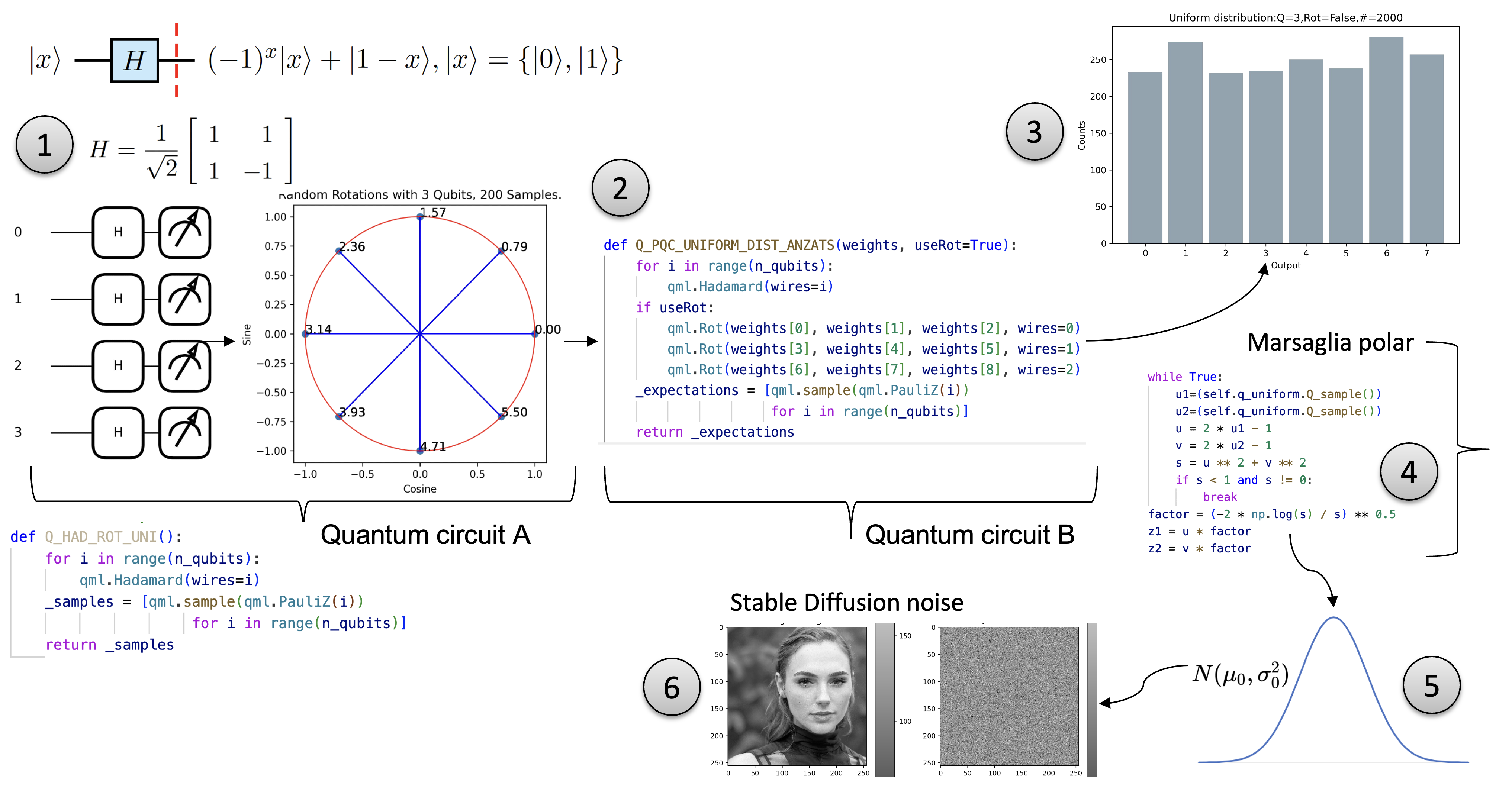
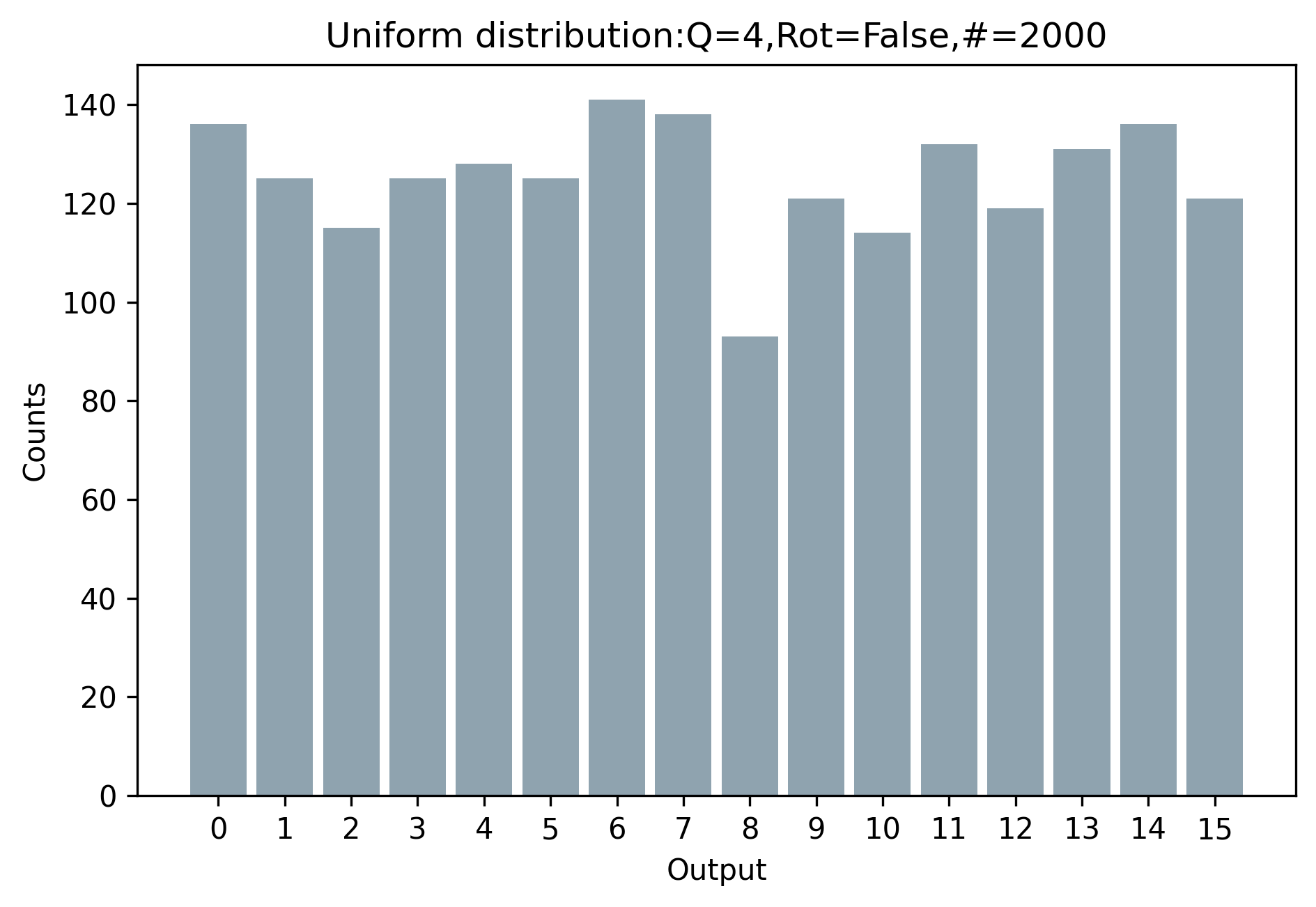
1 Utilizing N qubits, an initial non-parametric quantum circuit, founded on Hadamard transformations, engenders a uniform distribution across 2^N discrete values through sampled measurement outcomes, rather than expectation values. These outcomes are subsequently transmuted into equidistant angles, which are then channeled into a static quantum circuit that neither adapts nor learns, with the purpose of inducing stochastic rotations. 2 This static assembly, encompassing M>N qubits, functions as follows: a Hadamard gate is applied to each qubit, thus creating a superposition of states. Upon activation of the \texttt{useRot} flag, the circuit administers a rotation to every qubit, utilizing the \textbf{previously generated angles as the parameters for these rotations}. The output 3 from this circuit is then employed in the 4 Marsaglia polar method to transmute the uniform distribution into a zero-mean Gaussian 5. This transformation is achieved through the equation \(\mathbf{Z = \sqrt{-2\log U}\cos(2\pi V)}\), where U and V are two uniform random numbers, and by substituting our quantumly-generated uniform random bits for $U$ and $V$, we synthesize a source of quantum Gaussian random variables. 6 The Marsaglia polar method serves as a paradigmatic example of how quantum random bits can seamlessly supplant classical pseudo-random numbers in a Stable Diffusion (SD) model pipeline, specifically in the forward diffusion phase .
In this investigation, we introduce a method based on non-parametric quantum circuits for generating Gaussian Random Variables (GRVs).
This quantum-based methodology serves as an analogue to classical pseudorandom number generators (PRNGs),
such as those implemented in PyTorch's \textbf{torch.rand}. Importantly, our quantum Gaussian generator
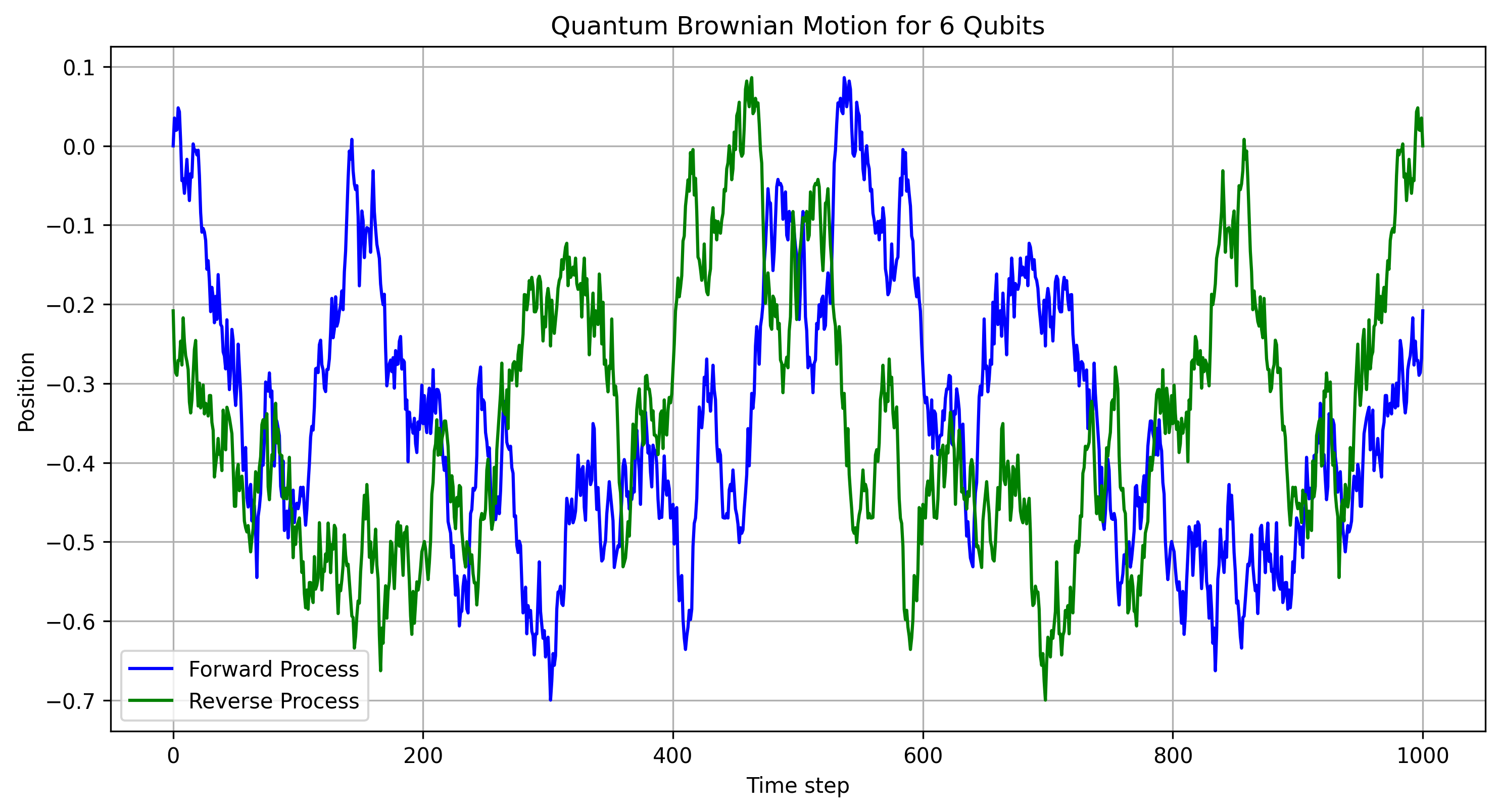
holds dual functionality: it offers a new avenue for simulating Stable Diffusion (SD) as well as Diffusion
Monte Carlo (DMC) techniques. Our approach stands in contrast to existing methods that employ parametric
quantum circuits, often in conjunction with variational quantum eigensolvers. These prevalent methods,
while effective for approximating the ground states of complex systems or learning intricate
probability distributions, necessitate a cumbersome and computationally demanding parameter
optimization phase. Our non-parametric approach eliminates this requirement. To facilitate the
integration of our methodology into existing computational frameworks, we unveil a Python library,
QonFusion.
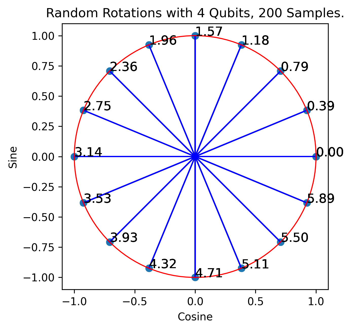
Initially, we employ \( N \) qubits in a non-parametric quantum circuit to produce a uniform
distribution over \( 2^N \) discrete outcomes:
The following animation illustrates the process. Each qubit randomly generates an angle, no entanglement is involved:
The resultant uniform PDF output is transformed into quantum rotations:
These are fed into the next quantum circuit:
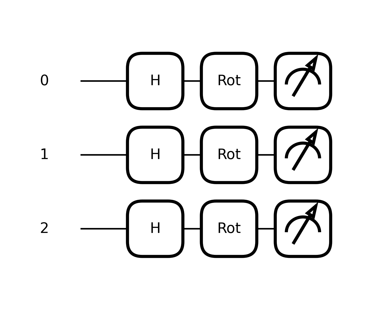
The mathematical representation of this 3-qubit quantum system undergoing a Hadamard transformation
followed by rotations can be formulated as follows:
Let's consider a numerical example for the system. We'll use the following rotation angles for each qubit:
The Hadamard gate \( H \) is represented as:
\[ H = \frac{1}{\sqrt{2}} \begin{pmatrix} 1 & 1 \\ 1 & -1 \end{pmatrix} \]And a general rotation \( U(\theta, \phi, \lambda) \) is given by:
\[ U(\theta, \phi, \lambda) = \begin{pmatrix} \cos(\frac{\theta}{2}) & -e^{i \lambda} \sin(\frac{\theta}{2}) \\ e^{i \phi} \sin(\frac{\theta}{2}) & e^{i (\phi + \lambda)} \cos(\frac{\theta}{2}) \end{pmatrix} \]First, we'll find the initial state \( |\psi_{\text{initial}}\rangle \) after applying the Hadamard gates:
\[ |\psi_{\text{initial}}\rangle = (H \otimes H \otimes H) |0\rangle^{\otimes 3} = \frac{1}{\sqrt{8}}(|000\rangle + |001\rangle + |010\rangle + |011\rangle + |100\rangle + |101\rangle + |110\rangle + |111\rangle) \]Next, we'll find the unitary operation \( U_{\text{total}} \) for the Hadamard and rotation gates:
\[ U_{\text{total}} = (U(\theta_1, \phi_1, \lambda_1) \otimes U(\theta_2, \phi_2, \lambda_2) \otimes U(\theta_3, \phi_3, \lambda_3)) \cdot (H \otimes H \otimes H) \]Finally, we'll find the final state \( |\psi_{\text{final}}\rangle \):
\[ |\psi_{\text{final}}\rangle = U_{\text{total}} |\psi_{\text{initial}}\rangle \]Calculating \( |\psi_{\text{final}}\rangle \) would involve the PannyLane library.
Here we provide the respective code snippet for the second circuit:
def Q_PQC_UNIFORM_DIST_ANZATS(weights, useRot=True):
    for i in range(n_qubits):
        qml.Hadamard(wires=i)
    if useRot:
        qml.Rot(weights[0], weights[1], weights[2], wires=0)
        qml.Rot(weights[3], weights[4], weights[5], wires=1)
        qml.Rot(weights[6], weights[7], weights[8], wires=2)
    _expectations = [qml.sample(qml.PauliZ(i))
                        for i in range(n_qubits)]
    return _expectations
Our focus is on sampling techniques.
The key difference between the expressions
\texttt{[qml.sample(qml.PauliZ(i)) for i in range(n\_qubits)]} and
\texttt{[qml.expval(qml.PauliZ(i)) for i in range(n\_qubits)]} lies
in the type of result they produce.
The former yields a sampled measurement outcome, whereas the latter returns
the expectation value. Specifically, \texttt{qml.sample()}
performs a measurement on the qubit in the Pauli-Z basis, leading to the
collapse of the wavefunction and randomly returning either 0 or 1,
based on the inherent probabilities of the qubit state. Conversely,
\texttt{qml.expval()} calculates the expectation value \( \langle Z \rangle \) of the
Pauli-Z operator on the qubit, providing the average value
one would expect to measure, without causing the wavefunction to collapse.
In summary, \texttt{qml.sample()} gives a random measurement sample (0 or 1),
while \texttt{qml.expval()} delivers the expected average value of a measurement
(a value between 0 and 1). Sampling leads to the collapse of the quantum state,
whereas expectation values allow for continued quantum operations.
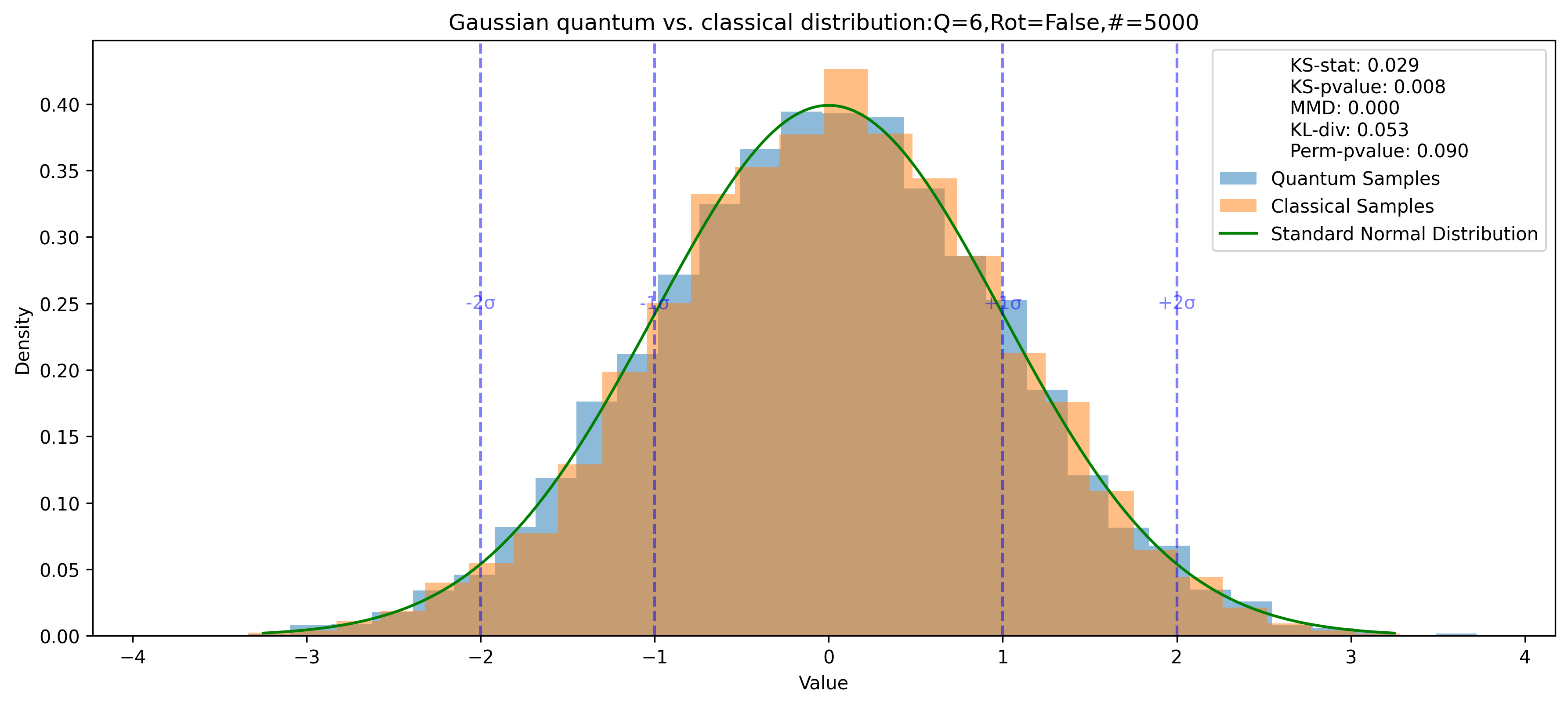
The quality of the quantum Gaussian distribution is validated using statistical tests [1], [2], [3] such as the Kolmogorov-Smirnov test as depicted in the table below.
| Test | Value |
|---|---|
| KS Statistic | 0.052 |
| KS P-Value | 0.124 |
| MMD | 0.001 |
| KL Divergence | 0.030 |
@misc{sk2023qdiffusion,
    title={Quantum Circuits for Gaussian Random Number Generation:
                            A Non-parametric Approach to the Stable Diffusion Noise Corrupter.},
    author={Shlomo Kashani},
    year={2023},
    eprint={},
    archivePrefix={arXiv},
    primaryClass={}
}